This is a successor post to my previous post on Grokking Grokking. Here we present a heuristic argument as to why overparametrized neural networks appear to generalize in practice, and why this requires a substantial amount of overparametrization – i.e. the ability to easily memorize (sometimes called interpolate) the training set.
First, we review a key result by Mingard et al. The fundamental idea they demonstrated is that the reason neural networks generalize is because they have strong inductive biases towards learning smooth functions. Namely, if we randomly sample networks from some simple prior distribution over parameter space, then these networks typically output smooth functions \(f\) of the input data \(D\). This smoothness then leads to generalization since it naturally tends for small perturbations of the input to lead to similar classifications. Formally, following Mingard et al, we consider two distributions. First, the prior distribution of network parameter initializations \(p_{\text{init}}(f \| D)\). Samples from this distribution represent random draws of network parameters from some initialization distribution. Secondly, there is the posterior of network parameters after training \(f_{\text{opt}}(f \| D)\). We can consider a sample from this distribution to consist of a fully trained network which achieves 0 training loss – i.e. it can perfectly interpolate the training data. Mingard et al demonstrate two key points empirically:
1.) That ranndomly initialized neural network functions are smooth. That is \(f(D,\theta)\) where the neural network parameters \(\theta\) are sampled from \(p_{\text{init}}(\theta)\) is a smooth function which thus generalizes. 2.) That the posterior distribution \(p_{\text{opt}}(f \| D)\) is close to the prior distribution \(p_{\text{init}}(f \| D)\) to first order. Thus trained networks also tend to learn smooth functions that generalize.
What this means is that previous arguments that overparametrized generalization is due to SGD having some specific inductive bias towards generalization is unnecessary. SGD can just find some optimum sampled from \(p_{\text{opt}}(f \| D)\) and this sample is likely to be close to a function sampled from the prior, and thus the function is highly likely to be smooth. Mingard et al demonstrate that this effect occurs empirically across a wide range of neural network architectures and initializations. A key question which remains unanswered, however, is why the posterior sampled by SGD is similar to the prior to first order and why this effect only appears to occur with a highly overparametrized neural network. Intuitively, the similarity between posterior and prior is not what we should expect. Surely, if SGD is optimizing the neural network significantly – i.e. over thousands of training iterations, and taking the network from random guessing to perfect memorization of the training set – then we should expect the parameters it finds to form a significantly different distribution from the parameters it was initialized with.
We argue that this intuition that the parameter posterior should differ substantially from the prior is true in the underparametrized, and slightly overparametrized case, but becomes increasingly untrue as the network becomes increasingly overparametrized and in the limit the posterior and prior become identical. Here we present a heuristic argument but aim to flesh this out more formally in later work.
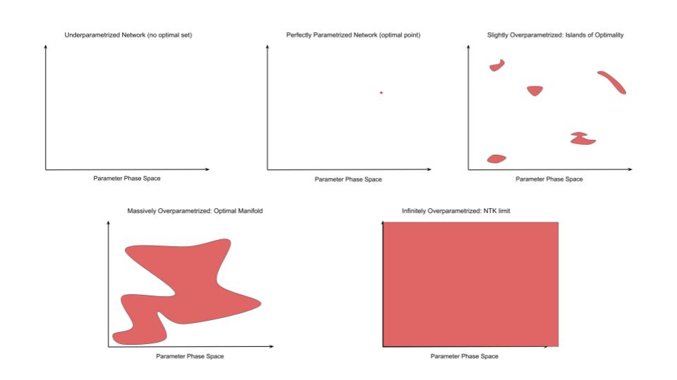
The key intuition arises from considering the optimal set of solutions in parameter space as overparametrization increases. This is explained in the previous blog post. This concept is easiest to understand in the context of the linear equations we solved in highschool. We consider a set of linear simultaneous equations with P equations and N unknowns. If \(N > P\) then we more unknowns than equations and there is no exact solution. This corresponds to the underparametrized case where the best we can do is make an approximation that mininimizes some loss function such as the squared error. In the case where \(N = P\), then we can solve the equation exactly. This is usually considered the ideal solution in the context of linear equations, and corresponds to an exactly overparametrized model such that there is exactly one solution which perfectly memorizes the training data. Finally, if \(P > N\), then we have many more parameters than unknowns and we have many equivalent solutions to the equations. Specifically, for every extra \(P > N\) we gain an additional dimension of solutions which are all optimal. This corresponds to an overparametrized model with many optimal parameter settings which can perfectly memorize the training data. We call this set of parameter settings the optimal set.

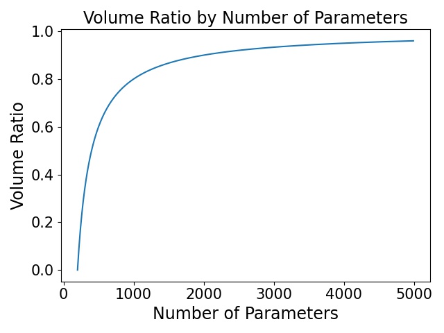
In the linear case, we gain one additional dimension of optimality per parameter more than N. That is, we can think of the ratio of the volume of the optimal set to the total parameter space as: \(\frac{(P - N)}{P}\) which we see increases logarithmically towards 1 as P increases (see graph). Explicitly computing this ratio for deep neural networks needs to be worked out rigorously in practice.

The key thing to realize is that, in the language of Mingard et al, the volume of the optimal set corresponds to the posterior \(p_{\text{opt}}(f \| D)\) while the volume of the total parameter space approximately corresponds to the prior \(p_{\text{init}}(f \| D)\) over the parameters (assuming a uniform prior and posterior over the sets). This means that we can express the average logarithm of this ratio as the KL divergence between the prior and posterior \(KL[\text{posterior} \|\| \text{prior}]\) and in general the two quantities are highly related.
However, as in the linear case, as the degree of overparametrizaiton increases, we should expect the ratio of optimal set to the parameter volume to increase. This means that the KL divergence between posterior and prior must decrease and hence the posterior sampled by SGD becomes increasingly similar to the prior. This then provides an exact reason for why we should expect this effect to occur in practice.
Thus far we have provided just a heuristic argument for why this is true. There are many mathematical details that need to be fleshed out to make such an argument rigorous, as well as many interesting questions which extends from these heuristics. These include: 1.) Can we quantify the size of the optimal set relative to the total volume of parameter space and how this ratio changes according to degree of overparametrization 2.) Can we quantify the average distance from a reasonable initialization to the optimal set as it varies with degree of overparametrization 3.) Can we obtain a quantitive measure of the statistical ‘averageness’ of regions of the optimal set as it varies with overparametrization 4.) Our argument suggests that, in the highly overparametrized regime, the standard bounds from VC theory, which typically utilize worst case scenarios are vastly pessimistic and, as such, become vacuous in practice. Instead we should be considering average case generalization bounds. And that these average case bounds should become asymptotically tight as the degree of overparametrization tends to infinity. Are there / can we prove any rigorous bounds on the average case generalization behaviour of neural networks?
Our argument also provides an explanation for why this effect should be highly robust across optimizers and architectures. In fact, our argument holds for essentially any architecture as the number of parameters increases. The effect of architecture and optimizer is essentially just to define non-uniform priors and posteriors over the volumes in parameter space.
I plan to be working on this mathematical theory over the coming months but don’t have much of the maths background needed for proving results of this type. If anybody is interested and has such a background please reach out as I’d be happy to collaborate.